Anyone can make an election model

Building the Economist’s election forecast model in pymc3

I’ve never been very interested in politics. But like many others, I got caught up in the hubbub of this past election, especially given the high stakes involved. So I started paying more attention to forecasts from FiveThirtyEight and TheEconomist, followed Nate Silver on Twitter, and even got distracted by the popcorn drama flame war between the two election forecasters.

As well as reading posts by Andrew Gelman – for anyone curious, he has some fantastic posts digging into the components of the Economist model.

All this also got me curious as to how hard it would be to build one of their forecast models.

As it turns out, it’s not too difficult. I can’t speak about FiveThirtyEight’s model, but the folks at the Economist were kind of enough to put their model and datasets on Github, so anyone can go through their code and reverse-engineer it. Their model is built in R and Stan – I have no familiarity in Stan, but I thought it would be a fun project to try to rebuild their model in Python with pymc3.

How the model works

If you just take a look at their repo, they state the inspiration for the model

“Improving on Pierre Kremp’s implementation of Drew Linzer’s dynamic linear model for election forecasting”

And if you follow the links, you get directed to this paper, which seems to be the source model. (By the way, I encourage anyone interested to read the actual paper, the math in it is pretty accessible and it’s a nice application of Bayesian modeling.)

This is the model we’re going to build in pymc3. It’s not exactly the Economist’s model, but it’s close enough – their model is a bit more complicated by trying to account include between state covariances and polling biases. I’m not a real election forecaster, so we’re going to keep it simple.

At it’s core, the model has two main components:

1. A “structural” forecast, based on economic and political factors
2. A series of random walks describing the trends of voter preferences throughout time.

We’ll break these down one by one:

1. Structural Forecast

The structural model turns out based on an earlier model known as Time for a Change, described in this paper. This model predicts the current presidential incumbent’s vote percentage from a regression on a few features, including the incumbent’s June approval rating and the latest Q2 GDP growth numbers. I don’t have much background on this, but supposedly this model worked well in the past.

There’s nothing Bayesian about this model – instead we’ll be using it’s prediction as a prior for the larger model

2. Voter Preference Trends

For this part, we assume that trends in state-level preferences are governed by two random walks: a national component \(\alpha\), and a state-specific component \(\beta_{s}\). Combining those, we end up with a stochastic variable representing state level preferences at time t.

(Logit is used to restrict the variable between 0 and 1)

The trend for \(\pi_{s,\ t}\) determines results in the polling data, given by the relationship

The \(\beta\) and \(\alpha\) parameters are then modeled as a reverse random walk (I didn’t know you can do this!), given by:

The structural forecast is used to set the time T (election date) prior on the state-level preferences \(\beta_{s,\ t}\) If you think about it, this makes sense, since the structural forecast is trying to predict what the preferences are going to be on the election date, not 90 or so days before.

\(\alpha\) is given a prior at time T of 0 – the reason being that on election day, we expect votes to be determined purely by state-specific effects. If you look at the paper, they describe it as “a national-level effect detects systematic departures from Beta”.

Even though this is now a reverse random walk, I think intuitively we can still think of this as a normal random walk. The key thing is that the prior is just on the last time step instead of the first. You can think this as saying, absent any data, we expect voter preferences on election day (day T) to be what we forecasted from the fundamentals model.

Show me the code

Let’s apply this model on data from the 2012 election. Here we’re just fitting a simple linear regression model Incumbent vote ~ June Approval Rates + Q2 GDP Growth

import pandas as pd
from sklearn.linear_model import LinearRegression

def fit_fundamentals_model():
    df = pd.read_csv('data/abramowitz_data.csv')
    train_df = df[df['year'] < 2012]
    model = LinearRegression(fit_intercept=True)
    X, y = train_df[['juneapp', 'q2gdp']], df['incvote']
    model.fit(X, y)
    print('R-squared: %f' % model.score(X, y))
    inc_prediction = model.predict(df[df['year']==2008][['juneapp', 'q2gdp']])[0]
    print('incumbent prediction: %f' % inc_prediction)

    prior = (100 - inc_prediction) / 100.  # Taking inverse and normalizing since we're predicting for Obama
    print('national prior %f' % prior)
    return prior

prior = fit_fundamentals_model() # 0.558804

And we get our prior of 55.8%.

To get state-specific priors, we can incorporate state level differences between % votes for Obama in the previous 2008 election, and apply those differences on priors

votes = pd.read_csv('data/2008.csv')  # 2008 results data
votes['vote_share'] = votes['total_count'] / votes['total_count'].sum()
votes['obama_diff'] = votes['obama'] - (votes['obama_count'].sum() / votes['total_count'].sum())

# states is an array of state names
state_weights = np.asarray([votes[votes['state']==s]['vote_share'].iloc[0] for s in states])
state_prior = np.asarray([votes[votes['state']==s]['obama_diff'].iloc[0] + prior for s in states])
# array([0.41770557, 0.41770557, 0.47770557, 0.63770557, 0.56770557,
#        0.63770557, 0.53770557, 0.49770557, 0.74770557, 0.56770557,
#        0.38770557, 0.64770557, 0.52770557, 0.43770557, 0.42770557,
#        0.64770557, 0.64770557, 0.60770557, 0.59770557, 0.56770557,
#        0.51770557, 0.49770557, 0.52770557, 0.47770557, 0.44770557,
#        0.56770557, 0.59770557, 0.59770557, 0.57770557, 0.65770557,
#        0.54770557, 0.36770557, 0.59770557, 0.56770557, 0.65770557,
#        0.47770557, 0.44770557, 0.46770557, 0.36770557, 0.55770557,
#        0.69770557, 0.60770557, 0.58770557, 0.45770557])

state_weights will come into play later.

def get_polls():
    polls = pd.read_csv('data/all_polls_2012.csv')
    print('polls.shape', polls.shape)
    polls['end.date'] = pd.to_datetime(polls['end.date'])
    polls = polls[polls['end.date'] >= '2012-08-01']
    election_date = pd.Timestamp('2012-11-06')

    # Breaking out data into 5 day intervals
    polls['days_to_election'] = polls['end.date'].apply(lambda x: (election_date - x).days)
    polls['day_idx'] = polls['days_to_election'].apply(lambda x: x//5)

    polls = polls[polls['number.of.observations'].notnull()]
    polls['number.of.observations'] = polls['number.of.observations'].astype(int)
    polls['obama'] = polls['obama'].astype(int)
    polls['obama_share'] = ((polls['obama'] / 100.) * polls['number.of.observations']).astype(int)

    state_polls = polls[polls['state'] != '--']
    national_polls = polls[polls['state'] == '--']
    return state_polls, national_polls

state_polls, national_polls = get_polls()

There are both national and state polls in this dataset. National polls will be handled differently.

Then we just need to fit our Bayesian model to polling data.

with pm.Model() as model:
    s_idx = pm.Data('state_idx', state_polls['state_idx'])
    s_day = pm.Data('state_day', state_polls['day_idx'])
    n_day = pm.Data('national_day', national_polls['day_idx'])

    # Defining state priors
    s_prior = pm.Normal('state_prior', 0, 1, shape=num_states) + state_prior
    s_sigma = pm.HalfCauchy('state_sigma', 1, shape=num_states)
    s_walk = GaussianRandomWalk('state_walk', sigma=1, shape=(num_days, num_states))

    # Defining national effect priors
    n_walk = GaussianRandomWalk('nation_walk', sigma=1, shape=num_days)
    n_sigma = pm.HalfCauchy('nation_sigma', 1)

    # Combining state and national effects
    state_effect = pm.Deterministic('state_effect',
                                    pm.math.invlogit(
                                        ((s_walk * s_sigma) + s_prior) + \
                                        tt.stack(n_sigma * n_walk).T
                                    ))

    # State polls
    state_poll_results = pm.Binomial('state_poll_results',
                                     n=state_polls['two_party_votes'],
                                     p=state_effect[s_day, s_idx],
                                     observed=state_polls['obama_votes'])

    # National polls
    weighted_national_effects = pm.Deterministic('weighted_national_effects', (state_effect * state_weights).sum(axis=1) / state_weights.sum())
    national_poll_results = pm.Binomial('national_poll_results',
                                        n=national_polls['two_party_votes'],
                                        p=weighted_national_effects[n_day],
                                        observed=national_polls['obama_votes'])

Note the part weighted_national_effects = pm.Deterministic(... (state_effect * state_weights)...), this is how the model is fit on national polling data.

Once the model is fit in pymc3, we can generate some charts from the resulting trace, such as the one below that shows the evolution state-level voter preference for Obama over time. The blue line is what the model learned, and the red dots are the results from the state polls.

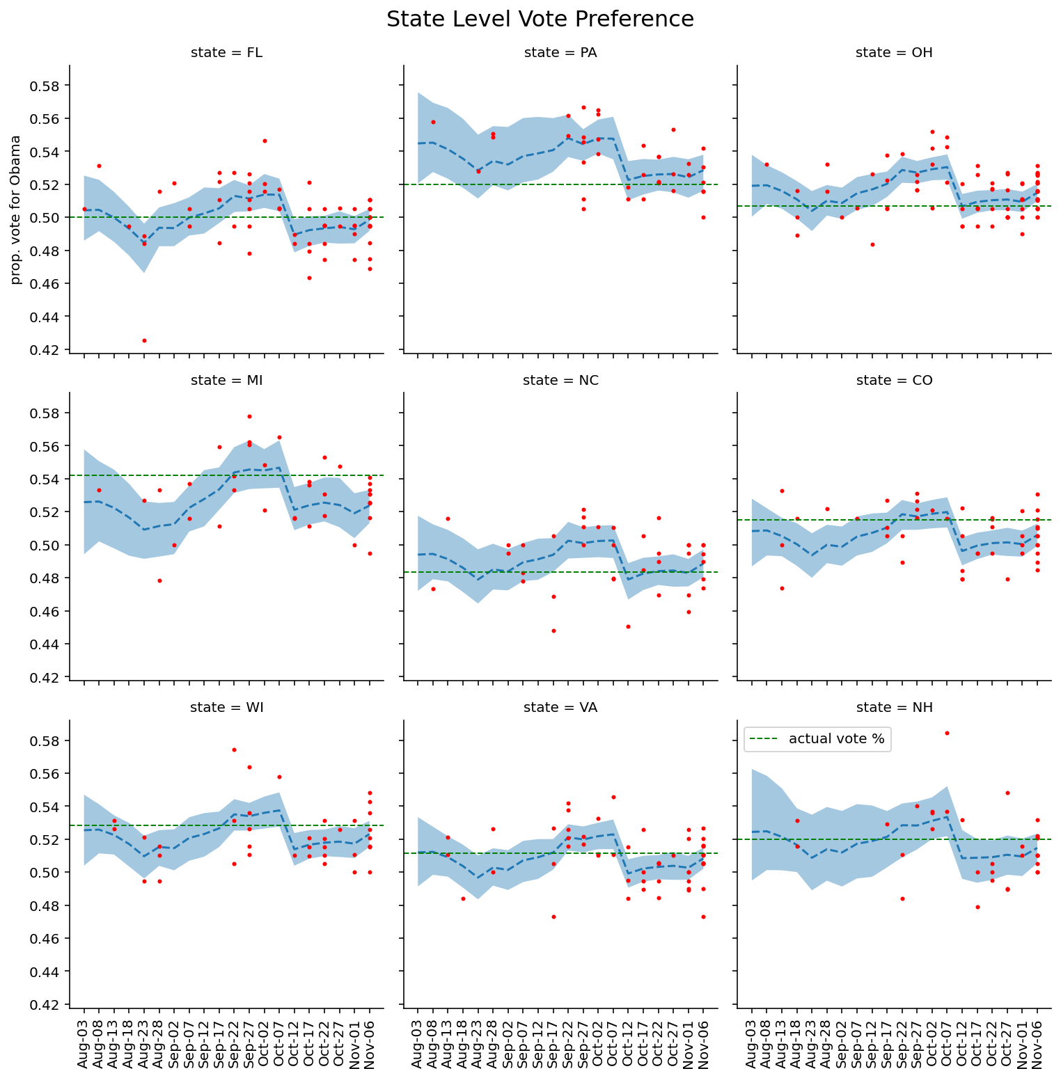
Interestingly, we see a drop in Obama favorability around the beginning of October, right around the time of the Oct 3 debate, in which Romney supposedly performed well. Also, all the state-level preferences seem to have the same trend – if you look closely, you can see they all peak in fall on the same dates, which speaks to how powerful the national level effect (\(\alpha_t\)) is in this model. (You can see the same pattern on the Economist’s github)

From the trace, we can also get samples of the final vote probability for each state, and use that to generate the final election win probabilities.

total_effect = trace['state_effect']
total_votes_arr = []
for i in range(total_effect.shape[0]):
    total_votes = 0
    for j, p in enumerate(total_effect[i, -1]):
        state = states[j]
        if p > .5:
            total_votes += electoral_votes[state]
    total_votes_arr.append(total_votes)
total_votes_arr = np.asarray(total_votes_arr)

plt.figure(figsize=[10, 6])
ax = plt.subplot(111)
plt.hist(total_votes_arr, bins=50, alpha=.8)
win_pct = (total_votes_arr >= 270).sum() / float(len(total_votes_arr))
ax.axvline(270, ls='--', c='r')
ax.set_title('Obama Win Probability:  %d%%' % (win_pct * 100), fontsize=16)

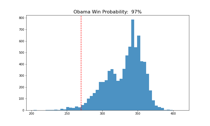
And that’s it! Overall it wasn’t too complicated, the most annoying part was waiting for the MCMC sampler to converge. I don’t get use pymc3 much in my day job, so it was nice to play around with it some more.

Addendum

• Again, huge props goes to the Economist for releasing and open sourcing their model. Without their documentation and code to guide me, I wouldn’t be able to do this post at all.
• I should emphasize, getting the MCMC sampler to run a few thousand samples is actually pretty annoying. I don’t remember exactly, but I think getting 10K samples took over 40 minutes. The dataset really isn’t that large, so I’m guessing this is just from the complexity of fitting a 51 random walk variables.